Navigating Uncertainty: Powering Business Insights with Simulations and Modeling in Excel
Imagine making crucial business decisions not just on past data, but on a map of all plausible futures. That's the power of Simulations and Modeling with Random Data in Excel – a robust technique that allows you to mimic real-world unpredictability, understand potential outcomes, and assess risks, even when historical data is scarce or nonexistent. Whether you're projecting next quarter's sales, stress-testing a new business plan, or estimating project timelines, Excel's simulation capabilities can transform guesswork into informed strategy.
At a Glance: What You'll Master in This Guide
- Why Simulate? Grasp the core benefits: better forecasts, smarter risk assessment, optimized strategies.
- Excel's Random Foundation: Leverage
RAND()andRANDBETWEEN()for basic unpredictability. - Modeling Reality with Distributions: Learn to simulate data that behaves like real-world phenomena, especially the common Normal (Bell Curve) Distribution.
- The Monte Carlo Method Demystified: Understand and implement complex simulations to explore thousands of potential scenarios.
- Practical Application: Walk through a step-by-step example of forecasting new product launch profits.
- Boosting Accuracy: Discover techniques to refine your simulations and generate more reliable insights.
Why Guess When You Can Simulate? The Edge of Data Modeling
In business, certainty is a rare commodity. Market shifts, customer behavior, supply chain disruptions – they all introduce variables that can make or break your plans. Traditional forecasting often provides single-point estimates, offering little insight into the range of possibilities or the probability of different outcomes.
This is where data simulation shines. By generating random numbers that reflect the inherent variability of your business environment, you can construct models that paint a much richer picture. You're not just predicting a future; you're exploring many plausible futures, each with its own likelihood.
Consider these powerful applications:
- Forecasting Performance: Instead of a single sales target, simulate a range of possible sales figures, profit margins, or project costs. This reveals not just an expected value, but the best-case, worst-case, and most likely scenarios.
- Assessing Risk: Quantify the probability of undesirable outcomes, such as the chance of losing money on a new product launch or exceeding a project budget.
- Testing Systems & Operations: Model customer call volumes, website traffic, or production line throughput to plan capacity and optimize resource allocation before issues arise.
- Optimizing Strategy: Compare various business strategies under different market conditions to identify the most robust and resilient approach.
At its heart, simulation helps you answer the crucial "what if?" questions with data-driven confidence, turning uncertainty into a strategic advantage.
The Building Blocks: Injecting Randomness into Excel
The foundation of any simulation in Excel lies in its ability to generate random numbers. While seemingly simple, mastering these core functions is critical for creating dynamic, realistic models.
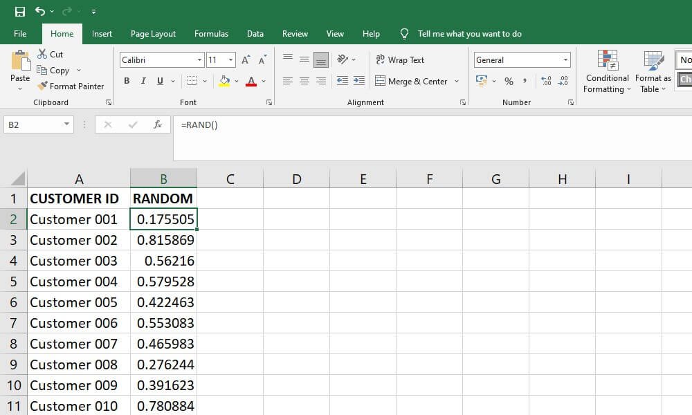
RAND(): Your Gateway to Random Decimals
The RAND() function is your simplest tool for introducing unpredictability.
- What it does: Generates a random decimal number greater than or equal to 0 and less than 1 (0 <= x < 1).
- Formula:
=RAND() - Example: If you type
=RAND()into a cell, you might see0.1284,0.9452, or0.5003. - Scaling
RAND(): You can adaptRAND()to produce random decimals within any range. For example, to get a random decimal between 50 and 100:=50 + (100-50)*RAND(). This formula takes the lower bound (50) and adds a random fraction of the range's width (100-50).
RANDBETWEEN(): For Whole Number Randomness
When your data naturally occurs as whole numbers – like the roll of a die or the number of customers – RANDBETWEEN() is your go-to function.
- What it does: Generates a random integer between two specified numbers (inclusive).
- Formula:
=RANDBETWEEN(bottom, top) - Example (Dice Roll): To simulate the roll of a standard six-sided die, use
=RANDBETWEEN(1, 6). - Example (Daily Sign-ups): If your daily website sign-ups typically range from 25 to 75, you can simulate this with
=RANDBETWEEN(25, 75).
The Volatility Trap (and How to Freeze It)
A critical characteristic of both RAND() and RANDBETWEEN() is their volatility. This means they recalculate and generate a new random number every time you make a change to your spreadsheet, press F9, or perform certain actions. While this is great for running many simulations, it can be frustrating if you need a static set of random numbers for analysis.
How to "Freeze" Random Data:
- Select the cells containing your
RAND()orRANDBETWEEN()formulas. - Copy them (
Ctrl+CorCmd+C). - Right-click on the same cells (or a new location if you want to preserve the formulas).
- Choose
Paste Special > Values(the icon that looks like a clipboard with "123" on it).
This action replaces the formulas with their current numerical results, effectively freezing your random data. For more on how to quickly generate random numbers and other uses, you might find this guide on how to generate random numbers in Excel helpful.
Beyond Uniform: Simulating Real-World Distributions (The Bell Curve)
While RAND() and RANDBETWEEN() are excellent for simple, uniformly distributed randomness (where every outcome in a range is equally likely), much of the real world doesn't work that way. Think about human heights, exam scores, or even monthly sales figures – values tend to cluster around an average, with fewer instances at the extremes. This pattern is often described by the Normal Distribution, commonly known as the "Bell Curve."
To simulate data that follows a Normal Distribution in Excel, you'll use the NORM.INV() function.
NORM.INV()Function: This function is typically used to find the value on a normal distribution curve for a given probability, mean, and standard deviation.- The Trick: By feeding
NORM.INV()a random probability (generated byRAND()), you can effectively "sample" a random value from a normally distributed dataset.
Understanding the Parameters:
probability: This is whereRAND()comes in. It provides a random decimal between 0 and 1, acting as a random percentile.mean: The average value of your dataset (the peak of the bell curve).standard_deviation: A measure of how spread out your data is. A larger standard deviation means the data points are more dispersed from the mean; a smaller one means they're clustered tightly around it.
Step-by-Step: Simulating Monthly Sales (Normal Distribution)
Let's say your average monthly sales are $150,000, and based on historical data or expert opinion, you estimate the standard deviation to be $20,000. You want to simulate 12 months of sales.
- Set up Your Parameters: In Excel, designate cells for your mean and standard deviation.
- Cell
F1:150000(Mean Sales) - Cell
F2:20000(Sales Standard Deviation)
- Input the Simulation Formula: In cell
A1(or your desired starting cell for the simulations), enter the formula:=NORM.INV(RAND(), $F$1, $F$2)
- Why
$? The dollar signs ($F$1,$F$2) create "absolute references." This means that when you drag the formula down, it will always refer back to these specific cells for the mean and standard deviation, rather than shifting relatively.
- Generate Your Data: Drag the fill handle (the small square at the bottom-right of cell
A1) down toA12to simulate 12 months of sales. Each cell will now show a different, normally distributed sales figure.
You'll observe that most of the simulated sales figures will hover around $150,000, with fewer numbers appearing at the very low or very high ends, perfectly mimicking a real-world bell curve.
Unleashing Predictive Power: Monte Carlo Simulations
While simulating a single variable like monthly sales is powerful, many business challenges involve multiple uncertain factors interacting with each other. This is where Monte Carlo Simulation comes into play. Named after the famous casino, this method involves running a simulation thousands, or even tens of thousands, of times. Each "run" uses different random inputs (drawn from their respective probability distributions) to generate a different outcome for your model.
By aggregating these thousands of outcomes, you can:
- Understand the full spectrum of possible results.
- Estimate the probability of specific outcomes (e.g., the chance of losing money).
- Identify the most likely range for a key metric.
Case Study: Forecasting Profit for a New Product Launch
Let's model the potential profit for a new product launch. Our basic profit equation is:Profit = (Units Sold × Price Per Unit) - (Variable Cost Per Unit × Units Sold) - Fixed Costs
Here are our assumptions, with key variables subject to randomness:
- Price Per Unit: $50 (fixed)
- Fixed Costs: $80,000 (fixed)
- Variable Cost Per Unit: Varies uniformly between $22 and $28 (meaning any value in this range is equally likely).
- Units Sold: Follows a Normal Distribution with a mean of 4,000 units and a standard deviation of 500 units.
Step-by-Step Implementation in Excel
1. Set Up Your Input Assumptions:
Dedicate a section of your spreadsheet to define all your fixed values and parameters for your random variables. This makes your model transparent and easy to adjust.
| Cell | Description | Value | Formula / Note |
|---|---|---|---|
| B2 | Price Per Unit | 50 | (Fixed) |
| B3 | Fixed Costs | 80000 | (Fixed) |
| B5 | Variable Cost (Low) | 22 | (Uniform Distribution parameter) |
| B6 | Variable Cost (High) | 28 | (Uniform Distribution parameter) |
| B7 | Units Sold (Mean) | 4000 | (Normal Distribution parameter) |
| B9 | Units Sold (Std Dev) | 500 | (Normal Distribution parameter) |
| 2. Build a Single Simulation Run: | |||
| Now, let's create the formulas for one iteration of our profit calculation, incorporating our random inputs. |
C5(Simulated Variable Cost):=$B$5 + ($B$6-$B$5)*RAND()- Explanation: This formula generates a random number uniformly distributed between our low ($22) and high ($28) variable cost assumptions.
C6(Simulated Units Sold):=NORM.INV(RAND(), $B$7, $B$9)- Explanation: This formula draws a random value for units sold from a normal distribution, using our defined mean (4,000) and standard deviation (500).
C8(Simulated Profit):=(C6*$B$2) - (C6*C5) - $B$3- Explanation: This calculates the profit for this single simulated scenario using our fixed price, simulated units sold, simulated variable cost, and fixed costs.
Every time you press F9 or make a change, theRAND()functions inC5andC6will recalculate, giving you a new profit outcome inC8.
3. Set Up for Thousands of Simulations Using a Data Table:
This is the magic trick for Monte Carlo in Excel. Excel's Data Table feature can perform thousands of recalculations of your model and collect the results, all without needing complex VBA code. - Create a Results Link: In cell
F1, link directly to your single simulated profit outcome:=C8. This tells the Data Table which output you want to capture from each simulation. - List Your Trial Numbers: In column
E, starting fromE2, create a list of numbers from 1 to 5000 (or more, depending on how many simulations you want). These numbers act as dummy inputs for the Data Table; their actual value doesn't matter, only that they are there. You can quickly generate this list by typing1inE2,2inE3, then selecting both and dragging down. - Select the Data Table Range: Select the entire range that includes your output link and your trial numbers. For 5,000 simulations, this would be
E1:F5001. - Activate Data Table: Go to the
Datatab on the Excel ribbon, thenWhat-If Analysis > Data Table.... - Configure Data Table:
- Row input cell: Leave this blank.
- Column input cell: Click on any empty cell outside your main model and the Data Table range. A good choice might be
D1. The Data Table uses this empty cell to feed each of your trial numbers (1, 2, 3...) back into the spreadsheet, forcing a recalculation each time. Since your random functions (RAND()) recalculate with any change, this effectively triggers a new simulation run for each number in your list. ClickOK.
Excel will now populate columnF(fromF2down toF5001) with 5,000 different simulated profit outcomes. Each result represents a unique combination of simulated variable costs and units sold.
4. Analyze Your Results:
With 5,000 profit outcomes, you can now perform powerful statistical analysis to gain true insights. - Average Profit:
=AVERAGE(F2:F5001) - Maximum Potential Profit:
=MAX(F2:F5001) - Maximum Potential Loss:
=MIN(F2:F5001) - Probability of Loss:
=COUNTIF(F2:F5001,"<0")/5000(Format as percentage). This tells you the percentage of simulations that resulted in a loss. - Profit at the 25th Percentile:
=PERCENTILE(F2:F5001, 0.25)– This means there's a 25% chance that your profit will be this value or lower. - Visualize with a Histogram: Select your profit outcomes in column
F. Go toInsert > Charts > Statistical Chart > Histogram. This visual representation will show you the distribution of your profits, highlighting the most likely range and the shape of the outcomes.
This comprehensive analysis provides far more insight than a single-point estimate. You're now equipped to answer questions like: "What's the most likely profit range?" or "What's the worst-case scenario, and how often might it occur?"
Refining Your Insights: Boosting Simulation Accuracy
While Monte Carlo in Excel is powerful, its accuracy and utility hinge on a few critical considerations. To ensure your simulations provide reliable, actionable insights, consider these refinement strategies:
1. Increase the Number of Simulations
The more times you run your simulation, the more closely the distribution of your outcomes will resemble the true underlying probability distribution of your model.
- The Law of Large Numbers: This statistical principle states that as the number of trials increases, the average of the results obtained from a large number of trials should be close to the expected value, and will tend to become closer as more trials are performed.
- Excel's Limits: For models with few variables, a few thousand simulations (like our 5,000 example) might be sufficient. However, for highly complex financial models or analyses requiring extreme precision, you might need tens of thousands or even hundreds of thousands of simulations. At these scales, Excel's performance can degrade, and specialized simulation software, or programming languages like R or Python, might be more efficient.
2. Refine Your Input Distributions
The accuracy of your simulation is only as good as the accuracy of your input assumptions. Garbage in, garbage out, as the saying goes.
- Leverage Historical Data: If available, use past data to determine the mean, standard deviation, or shape of your input distributions. Don't just guess; let the numbers tell the story.
- Consult Domain Experts: When historical data is sparse (e.g., for a brand-new product), seek input from experienced professionals. Their qualitative insights can help you define reasonable ranges and central tendencies.
- Explore Other Distributions: Not everything fits a Normal or Uniform Distribution.
- Log-Normal: Good for values that can't be negative and tend to be skewed (e.g., stock prices, income).
- Beta: Useful for modeling probabilities or proportions (values between 0 and 1).
- Gamma: Often used for waiting times or financial claims.
Excel has functions likeLOGNORM.INV,BETA.INV, andGAMMA.INVthat work similarly toNORM.INVwhen combined withRAND(). - Custom Distributions: If your data follows a unique, non-standard pattern, you might create a custom lookup table combined with
VLOOKUPandRAND()to sample from it.
3. Conduct Sensitivity Analysis
While not strictly a Monte Carlo technique, sensitivity analysis is a crucial complement. It helps you understand which input variables have the greatest impact on your model's output.
- How it works: Systematically vary one input parameter (e.g., the standard deviation of units sold) while holding all other inputs constant, and observe the change in your output (e.g., average profit).
- Why it matters: If your model's output is highly sensitive to a specific input, it tells you two things:
- That input's probability distribution needs to be as accurate as possible.
- That input represents a key risk or opportunity that warrants closer management or strategic focus.
By focusing your data gathering and analysis efforts on the most sensitive variables, you can significantly enhance the robustness and reliability of your simulation results.
Common Questions and Pitfalls
Simulations, while powerful, can sometimes lead to confusion. Here are answers to common questions and how to avoid typical pitfalls:
"My simulated numbers keep changing! How do I get them to stop?"
This is the volatility of RAND() and RANDBETWEEN() at work. As discussed, use Copy then Paste Special > Values to freeze your results for analysis. If you want to rerun a simulation, simply generate new random numbers (e.g., by pressing F9 or making a minor edit) and then freeze them again.
"How many simulations are enough?"
There's no single magic number. It depends on:
- Model Complexity: More complex models with many interacting random variables generally need more simulations.
- Desired Precision: If you need highly precise probability estimates, you'll need more runs.
- Variability of Inputs: Inputs with high variability require more simulations to capture the full range of possibilities.
- Computational Resources: Excel can slow down significantly with tens of thousands of formulas.
A good practice is to run a small number of simulations (e.g., 1,000), then increase it (e.g., to 5,000, then 10,000). If the key metrics (average, probabilities) stop changing significantly between runs, you're likely in a good range.
"My histogram looks weird – it's not a smooth curve."
This could be due to: - Too Few Bins: Excel's default histogram settings might use too few bins, making the distribution appear blocky. Adjust the number of bins to create a smoother representation.
- Too Few Simulations: With a small number of simulations, the random noise might dominate, preventing a smooth curve. Increase the number of runs.
- Non-Normal Distribution: Perhaps your simulated variable isn't actually normally distributed. Double-check your
NORM.INVparameters or reconsider if a different distribution (e.g., uniform, skewed) might be more appropriate.
"Can I simulate discrete events or choices?"
Yes! For example, if there's a 30% chance a customer chooses Product A and 70% Product B:=IF(RAND()<=0.3, "Product A", "Product B")
You can extend this with nestedIFstatements orVLOOKUPagainst a probability distribution for multiple choices.
"Is Excel suitable for all Monte Carlo simulations?"
For many business applications, especially for learning and mid-range complexity, absolutely. Excel is accessible, visual, and powerful. However, for extremely large datasets, very complex interdependencies, or when highly specialized distributions are needed, dedicated statistical software or programming environments (like Python with libraries such as NumPy and SciPy, or R) offer greater speed, flexibility, and advanced features. Use Excel as a fantastic starting point and a powerful tool for many scenarios.
Turning Uncertainty into Strategy
Simulations and modeling with random data in Excel are more than just advanced spreadsheet tricks; they're a paradigm shift in how you approach decision-making. By embracing the inherent uncertainty of the business world rather than trying to ignore it, you move from reactive guessing to proactive, data-driven strategy.
You've learned how to inject randomness using RAND() and RANDBETWEEN(), how to mimic real-world distributions with NORM.INV(), and how to harness the immense power of Monte Carlo simulations to explore thousands of potential futures. You now possess the tools to not only predict what might happen but also how likely it is to happen, empowering you to make more resilient plans, assess risks with greater confidence, and ultimately, drive better business outcomes.
So, open Excel, embrace the random, and start simulating your way to clearer insights. The future may be uncertain, but your understanding of it doesn't have to be.